

The bullwhip effect in supply chain explained starts with a simple idea: small changes in end-customer demand turn into far larger swings in orders as they travel upstream. A 10% move at the shelf can become a 40% order change at your distributor and a 100% change at your resin supplier, because nobody upstream sees the customer. They see only the orders of the tier below them.
Jay Forrester named the phenomenon at MIT in 1961 while studying industrial systems, and Hau Lee and his co-authors later quantified it in 1997. It shows up in plastics, packaging, injection moulding and every other multi-tier operation that reorders on someone else’s forecast.
Table of Contents
- What Is the Bullwhip Effect in Supply Chain?
- How Does the Bullwhip Effect Move Through a Supply Chain?
- What Causes the Bullwhip Effect?
- What Is a Bullwhip Effect Example?
- How Do You Measure the Bullwhip Effect?
- How Can Manufacturers and Buyers Reduce the Bullwhip Effect?
- Which Control Is Most Effective for a Long Lead-Time Supply Chain?
- What Mistakes Make the Bullwhip Effect Worse?
- How Is the Bullwhip Effect Different from Normal Demand Volatility?
- Frequently Asked Questions
- What is the bullwhip effect in supply chain management?
- How is the bullwhip ratio calculated?
- What is the most common cause of the bullwhip effect?
- Does the bullwhip effect happen only in retail supply chains?
- How can procurement teams reduce bullwhip risk?
- Is the bullwhip effect always caused by inaccurate forecasts?
- Conclusion
What Is the Bullwhip Effect in Supply Chain?
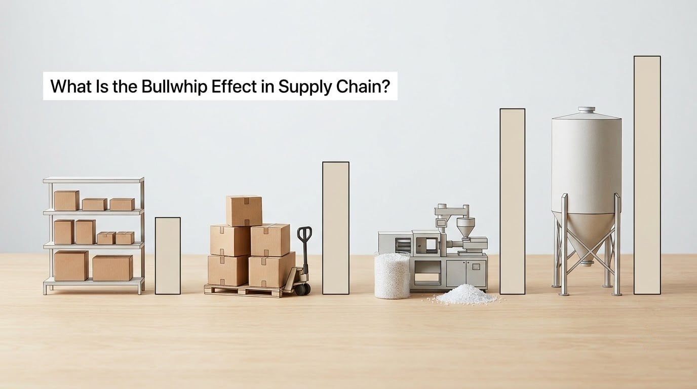
The bullwhip effect is the progressive amplification of demand variability as orders move upstream through the tiers of a supply chain. Also called the Forrester effect, it describes a situation where the further a tier sits from the final customer, the wilder its order swings become.
Two different things get confused here. Genuine demand variability is real and you cannot remove it — customers buy more coolers in July and fewer in January. Bullwhip is artificial: the orders do not match the demand that caused them. If the customer bought 1,000 pieces and your resin supplier ordered 2,000, the extra 1,000 came from someone guessing.
It is worth naming the shape of the thing. A steady line of demand at the customer end becomes a small wave at the distributor, a bigger wave at the manufacturer, and a violent swing at the raw material tier. The pattern looks exactly like a whip snapping, which is where the name comes from.
How Does the Bullwhip Effect Move Through a Supply Chain?
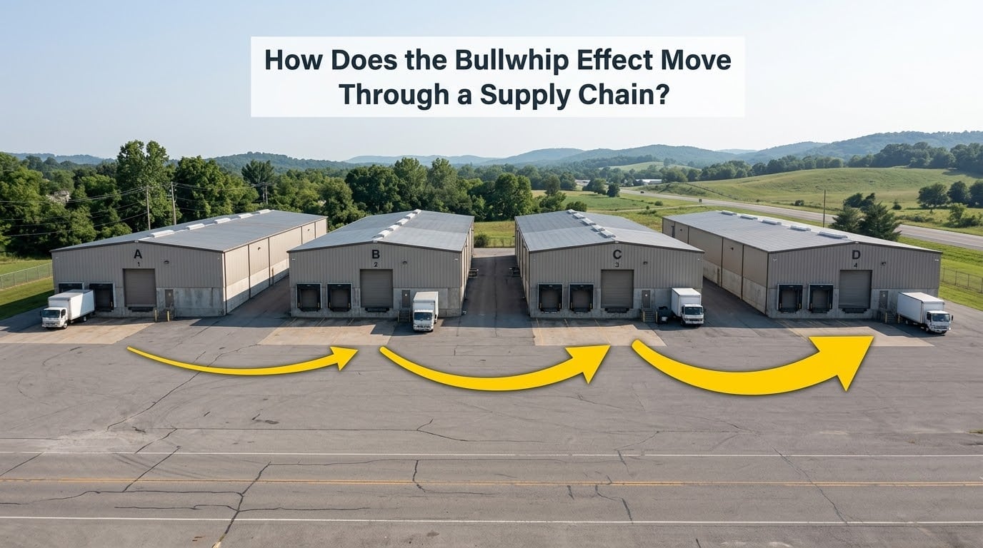
Amplification happens because each tier makes a locally reasonable decision using incomplete information. No tier is behaving badly. Each one is protecting itself against the tier above, and the sum of those self-protections becomes the whip.
- Demand changes at the shelf. A promotion lifts sales 10% and then sales fall back to normal.
- The distributor reacts to orders, not to sales. Its own customer, a regional wholesaler, jumped 20%. It has never seen the promotion.
- The manufacturer reacts to the distributor. A 20% order increase becomes a 40% production increase, because the plant assumes the trend will hold and adds buffer.
- The raw material supplier reacts to the manufacturer. A 40% order increase becomes a doubling of resin and additive orders, often with a lead time of weeks behind it.
- The correction travels back down. When customer demand returns to normal, the distributor’s orders fall 30%, the manufacturer cuts 50%, and the supplier may stop ordering entirely.
The signal always runs upstream, and it always returns amplified. Because lead time sits between the order and the delivery, each tier is ordering against a view of demand that is several weeks out of date. That delay is the fuel: without it, the wave flattens.
What Causes the Bullwhip Effect?
Demand forecasting errors
Exponential smoothing and similar methods respond to a rise by extrapolating it. A 10% increase gets forecast at 12% next month, then 14%, so the order curve drifts upward for reasons that have nothing to do with customers.
Order batching
Ordering small quantities often means paying more per piece and dealing with more inbound receipts, so buyers consolidate into weekly, monthly or quarterly windows. Batching turns a smooth signal into a step function, and the supplier sees a spike and a gap instead of a trend.
Price promotions and temporary discounts
You are not selling more, you are selling earlier. A distributor that buys 3,000 cases during a promotion holds 1,500 of them afterwards, and the next order drops by half. The upstream swing came from timing, not from consumption.
Long and variable lead times
A quoted lead time of four weeks that quietly becomes eight creates a systematic problem. Every tier must cover the gap with inventory, so each one orders more than it needs to survive the uncertainty.
Limited capacity and rationing
When a supplier can only ship part of what was ordered, buyers inflate their next order to protect their allocation. Suppliers see the inflated order as real demand. In shortages, the gap between ordered and received can exceed 50%.
No shared data and speculative buying
If the customer, distributor and manufacturer are working from different numbers with different time lags, nobody can reconcile them. Add the buyer who quietly adds 20% to every order because it is the only lever they have, and the distortion is guaranteed.
| Cause | Mechanism | Leading symptom | Fix |
|---|---|---|---|
| Forecast method | Extrapolates a recent rise | Order curve never flattens after a spike | Bias-corrected or intermittent forecasting |
| Order batching | Turns flow into steps | Supplier sees spike then silence | Smaller, more frequent releases |
| Promotions | Pulls demand forward | Post-promotion dip below plan | Share the promotion calendar upstream |
| Lead-time variance | Forces buffer inventory | Safety stock creeps upward each quarter | Commit to a lead time, then reduce it |
| Rationing | Inflates the next order | Ordered versus received gap | Allocate on history, communicate openly |
What Is a Bullwhip Effect Example?
Here is a standard multi-echelon case with real numbers. Steady customer demand of 1,000 pieces a month shifts by 10% in month four and then returns to baseline in month five.
| Tier | Steady demand | Month 4 response | Change | Month 5 response | Change |
|---|---|---|---|---|---|
| End customer | 1,000 | 1,100 | +10% | 1,000 | -9% |
| Distributor | 1,000 | 1,200 | +20% | 700 | -42% |
| Moulder | 1,000 | 1,400 | +40% | 500 | -64% |
| Resin supplier | 1,000 | 2,000 | +100% | 0 | -100% |
The customer barely moved. The resin supplier doubled production and then stopped, and a resin supplier who stops is a moulding plant that idles its lines. At the plant the consequence is concrete: an open mould for two runs of part number X, then nothing, then three emergency runs of Y to catch up on real demand.
The direction matters as much as the size. Over-ordering ties up cash in inventory, storage and work-in-progress, and the overage ages into obsolescence. Under-ordering means missed deliveries, emergency freight and overtime. Both directions cost money, and they cost it at the same time.
How Do You Measure the Bullwhip Effect?
You measure it with the bullwhip ratio, also called the bullwhip measure or variance ratio. It compares how much orders vary to how much demand varies over the same period. Above 1.0 means amplification; below 1.0 means the chain is smoothing things out, which is the goal.
The calculation divides the variance of orders received by a tier by the variance of the demand it is trying to serve:
Bullwhip ratio = Variance of orders / Variance of demand
Using four months of data for a distributor: customer demand runs 1,000, 1,200, 1,100 and 1,300 pieces, giving a variance of 12,500. The distributor’s own orders run 1,000, 1,500, 1,100 and 1,900, giving a variance of 126,875. The ratio is 126,875 divided by 12,500, which is about 10.1. Order variability is running roughly ten times demand variability at that tier.
A few practical points on measurement. Run the ratio over enough periods to include a seasonal cycle, because a quarter of data will flatter you. Compare a calm period with a volatile one, and calculate each separately; a stable stretch hides the problem entirely. And track the ratio per tier rather than across the whole chain, so you can see which relationship is distorting most.
If your tier-by-tier ratios climb as you move toward raw materials, you have measured the whip. That is your priority list for improvement, ranked by how much variability each tier is adding.
How Can Manufacturers and Buyers Reduce the Bullwhip Effect?
Share the demand signal, not just the forecast
The cheapest fix is free information. Give suppliers your actual consumption history, your promotion calendar and your project schedule, at a fixed cadence. Collaborative planning, forecasting and replenishment works when both sides commit to the same numbers and a review rhythm. Half the distortion disappears when a supplier can see that last month’s jump was a trade show, not a trend.
Smooth orders instead of spiking them
Replace one 500-piece order a quarter with five 100-piece orders. Larger and more frequent releases cut both transport cost and the supplier’s need to guess. On the plant side, a stable weekly cadence lets you run longer, fewer setups and keep a steadier crew.
Redesign replenishment and safety stock
Many safety stock policies add buffer on top of an already inflated forecast, which doubles the problem. Set safety stock from true demand variability and true lead-time variability, not from a forecast that already contains padding. If safety stock rises every quarter for no operational reason, you are absorbing a bullwhip you created yourself.
Shorten and stabilise lead times
Ask for a firm quoted lead time with a defined tolerance, and treat breaches as a supplier scorecard item. Physically shorter lead times help too: holding material handling systems for resin close to the press line, sizing hoppers to real consumption rates, and standardising grades so a changeover is minutes instead of hours.
Plan capacity against the signal, not the spike
Reserve supplier capacity in blocks that survive normal swings rather than committing to every monthly number. Add second sources for long lead-time components, and keep the bill of materials tight, because every extra grade and every extra supplier is another variable you cannot see.
Which Control Is Most Effective for a Long Lead-Time Supply Chain?
For long lead-time chains, order smoothing plus a firm lead-time commitment give the best return, because they attack the two mechanisms that make the whip large. Where the lead time runs past twelve weeks and the component is custom, capacity reservation and a redesigned bill of materials usually come next. Shorter and more frequent orders are the right lever when the problem is batching rather than lead time.
Where an item is expensive to bring onshore, the sourcing decision itself becomes a control. The tradeoffs are laid out in nearshoring versus offshoring tradeoffs, and the same logic applies to bringing a component in-house, covered in make or buy decision analysis.
No single control removes the variability. Order smoothing without information sharing just moves the distortion, and collaboration without firmer lead times leaves every tier guessing.
What Mistakes Make the Bullwhip Effect Worse?
- Treating one-off spikes as a new baseline. Correct by setting a trend window and requiring a minimum number of periods before raising the plan.
- Pasting the forecast straight into the order. A forecast is an estimate. Adjust it for known pipeline, promotions and project timing before releasing.
- Re-ordering during a shortage. Duplicate orders make a supply problem look like a demand surge. Confirm the original order is still open first.
- Letting safety stock absorb every surprise. Audit it quarterly; if it grew twice without a lead-time change, someone is hiding bullwhip in the buffer.
- Rescheduling constantly. Frequent schedule changes drive changeovers, scrap and overtime, and the cost lands inside your unit price. Freeze the schedule and let exceptions run as exceptions.
- Reading allocation as demand. What a supplier shipped under a cutback tells you nothing about what your customer wants. Track the order file for the real signal.
How Is the Bullwhip Effect Different from Normal Demand Volatility?
Normal demand variability is the customer moving. Bullwhip is your supply chain moving faster than the customer. A project-based moulder may see genuine 40% swings as customers commission new tools, and that demand is real, but if the resin supplier’s orders swing 80% in the same month, the gap between the two is the bullwhip.
The test is simple: compare the ratio of order variability to demand variability at each tier. Genuine volatility passes through the chain roughly intact or damped, and every tier sees the same shape at a different size. Amplification compounds, so each tier’s swing is larger than the one below it.
Seasonality deserves its own note, because seasonal demand and the bullwhip are often confused. A predictable summer peak needs capacity and inventory planning, not a fix to distortion. What makes it a bullwhip problem is the post-season collapse, where orders fall below true consumption and leave ageing stock behind.
Frequently Asked Questions
What is the bullwhip effect in supply chain management?
The bullwhip effect is the progressive amplification of demand variability as orders move upstream. A 10% change in end-customer sales can trigger a 20% order at the distributor, a 40% order at the manufacturer and a 100% order at the raw material supplier. Each tier reacts to the tier below rather than to real consumption, so orders swing far harder than the demand behind them.
How is the bullwhip ratio calculated?
Divide the variance of the orders a tier receives by the variance of the demand it serves, measured over the same number of periods. A ratio above 1.0 means amplification, and a ratio below 1.0 means the chain is smoothing demand. Calculate the ratio tier by tier so you can identify which relationship is adding the most variability.
What is the most common cause of the bullwhip effect?
Order batching is the most common single cause, closely followed by long and variable lead times. Buyers consolidate orders to cut purchasing effort and freight cost, which turns a smooth demand signal into a series of steps. The supplier reads each step as a genuine spike and inflates its own orders, adding variation at every tier.
Does the bullwhip effect happen only in retail supply chains?
No. Any multi-tier chain experiences it, including plastics, packaging and injection moulding operations. A moulder feeding distributors sees the same amplification as a consumer goods retailer, and the raw material tier sees the largest swing of all. The Beer distribution game reproduced it with four simple tiers and no retail involved.
How can procurement teams reduce bullwhip risk?
Share consumption history and the promotion calendar with key suppliers, then agree a firm lead time with a defined tolerance. Release smaller orders more often instead of quarterly batches, and confirm duplicate orders are open before raising new ones during a shortage. Track the bullwhip ratio per supplier so improvement is visible rather than assumed.
Is the bullwhip effect always caused by inaccurate forecasts?
No. Forecast error contributes, but order batching, promotions, rationing and lead-time variability can amplify orders even when every forecast is accurate. A promotion shifts buying earlier without changing consumption, so the forecast stays right while orders swing. That is why measuring the bullwhip ratio tells you more than forecast accuracy alone.
Conclusion
Start by measuring order-to-demand variability per tier, then fix the tier with the highest ratio before touching anything else. Share consumption history and the promotion calendar with that supplier, and commit to a lead time with a tolerance attached. After that, move from quarterly batches to smaller weekly releases and audit the safety stock that has been quietly absorbing the swings.
The bullwhip effect in supply chains is not a forecasting problem you solve with a better model. It is a behaviour problem you solve by shortening the feedback loop between what customers actually consume and what the tier above orders.