Economic Order Quantity Explained for Buyers: Formula (2026)

Economic order quantity explained for buyers in one line: EOQ is the order size that keeps your total inventory cost lowest by balancing the cost of raising a purchase order against the cost of holding the goods until they sell. You need three numbers to calculate it — how much you buy in a year, what one order costs you to place, and what one unit costs you to store for a year — and the formula turns them into a quantity.

Most small businesses guess their order sizes by feel. A buyer watches what sells, tops up the shelf, and repeats. That works until volume climbs, cash gets tight, and the same item sits in the back room for eleven months while the freight bill arrives every three weeks.

This guide walks through what EOQ actually decides, where each input comes from, a full worked example, and how to turn the result into a schedule you can hand to a colleague.

Table of Contents

• Economic Order Quantity Explained for Buyers: What It Actually Decides
  • What is economic order quantity in purchasing terms?
• EOQ Formula and Inputs
• How the EOQ Formula Works
• Economic Order Quantity Example for a Packaging Buyer
• How to Turn EOQ into an Order Schedule
• When a Buyer Should Not Use the Standard EOQ
• How to Adjust EOQ for Real Purchasing Conditions
  • How to calculate EOQ in a spreadsheet
• EOQ Versus Minimum Order Quantity and Reorder Point
• Key Assumptions and Common Calculation Errors
• A Buyer-Friendly EOQ Workflow
• Frequently Asked Questions
  • What should a buyer do if the EOQ is below the supplier MOQ?
  • How does EOQ handle demand that changes each month?
  • Should EOQ include supplier lead time in the formula?
  • How do volume discounts change the economic order quantity?
  • Can EOQ be used with a periodic inventory review system?
  • What is the easiest way to calculate EOQ in a spreadsheet?
• Conclusion: Start with a Testable EOQ Policy

Economic Order Quantity Explained for Buyers: What It Actually Decides

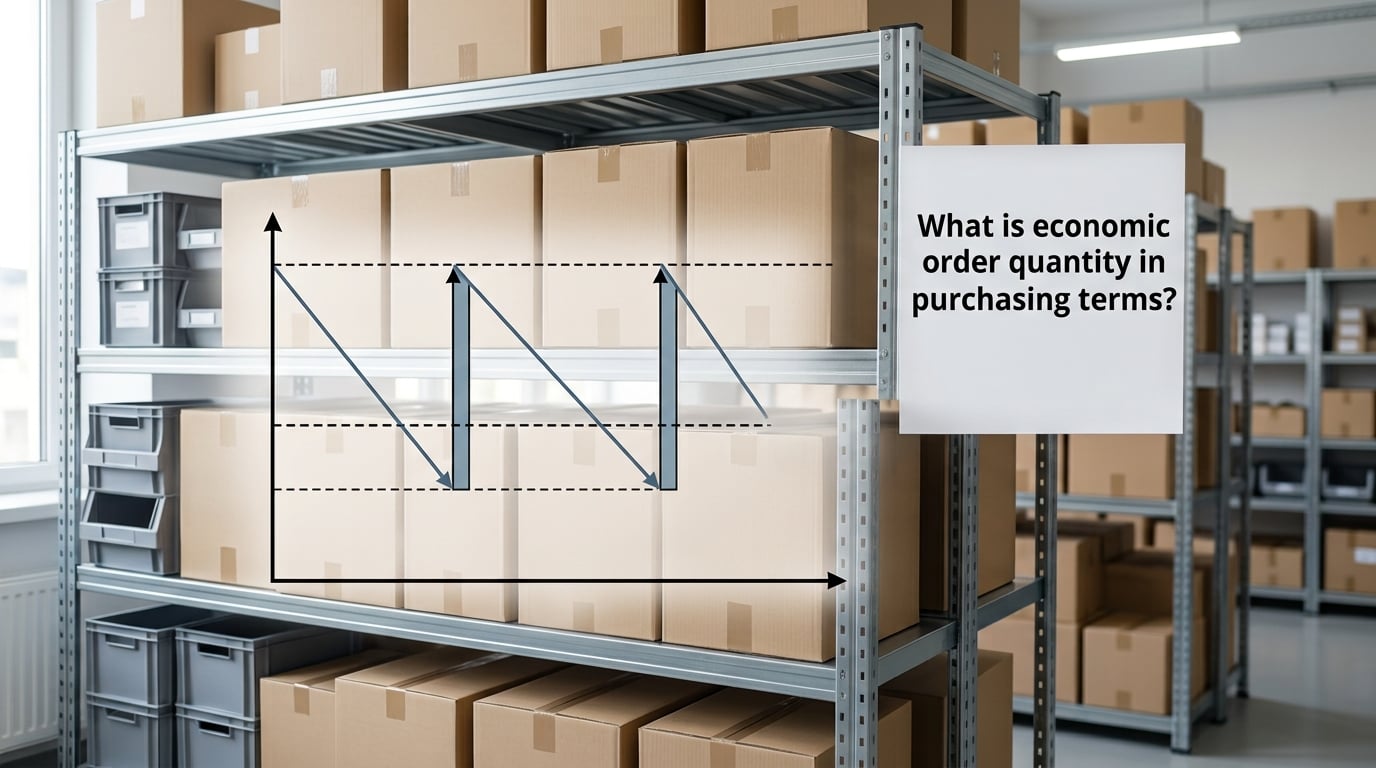
Economic order quantity is the number of units to buy in one single order so that ordering costs and holding costs add up to the smallest possible yearly total. It answers how much to order. It does not answer when to order — that is the reorder point’s job.

What is economic order quantity in purchasing terms?

In purchasing, economic order quantity is a sizing rule, not a purchasing decision. You run it per item, per period, and it returns a unit count. Ordering happens when inventory on hand falls to a trigger point, and EOQ decides the size of that order once it fires.

Two costs sit on opposite sides of every purchase. Ordering costs are the admin, freight setup, receiving labour and inspection you pay each time a PO goes out. Holding costs are storage space, insurance, insurance-adjacent handling, shrinkage, obsolescence and the capital tied up in goods sitting in your building.

Order small and you pay the ordering cost many times a year. Order large and you pay the holding cost on far more units than you need at once. EOQ is the point where the two curves cross and total cost is at its minimum.

Who uses it: wholesale distributors, retail buyers, marketplace sellers, restaurant and hospitality resupply, and manufacturing purchasing staff. What it never does is forecast demand, tell you whether to buy from a given supplier, or set a safety buffer.

EOQ Formula and Inputs

The formula is EOQ = √(2DS / H). Three inputs, one output, all three measured over the same twelve-month period.

√(2 × annual demand × ordering cost per order ÷ holding cost per unit per year)

EOQ variable table: what each symbol means and where a buyer finds it

Symbol	Name	Units	Where a buyer finds it
D	Annual demand	Units per year	Twelve months of units sold or issued, from your POS export, sales history or usage log
S	Ordering cost	Currency per order	Time to raise, send, receive and inspect one PO, priced at your labour rate, plus fixed freight and duty per shipment
H	Holding cost	Currency per unit per year	Annual cost of space, insurance, shrinkage, obsolescence and capital, expressed per unit on hand

Change one input and the answer moves predictably. Double annual demand and the order size grows by about 41 percent, because the square root halves the sensitivity. Double holding cost and the order size shrinks by about 29 percent. Ordering cost works the same way in the opposite direction: expensive to place means buy bigger, less often.

Units matter more than people expect. Monthly demand multiplied by twelve gives D in units per year; a holding cost quoted per month must be multiplied by twelve before it goes into the formula. Mixing months and years is the single most common arithmetic error I see.

How the EOQ Formula Works

Split the formula in half and each piece is a cost you already recognise.

The ordering side: annual demand divided by order quantity gives the number of orders you raise per year. Multiply that by S and you have your annual ordering cost. Order 5,000 units a year in 10,000-unit orders and you raise half an order a year, which is obviously wrong — and exactly what the calculation catches.

The holding side: stock arrives all at once, so average on-hand inventory is half the order quantity, Q ÷ 2. Multiply by H for your annual holding cost. This is why the model assumes a steady drip out to customers rather than everything leaving on day one.

Add the two together and you get total annual inventory cost. As Q grows, the ordering portion falls and the holding portion climbs. EOQ sits where they meet, and at that exact point the two costs are equal. That equality is a useful sanity check: if your ordering cost is four times your holding cost, your quantity is too small.

The square root is why the result is forgiving. Push demand up 50 percent and the optimal order size rises only about 22 percent. A slightly stale demand figure is therefore a small error, not a catastrophe.

Orders per year is just D ÷ Q. It tells you how many times a year someone has to raise a PO, chase a delivery date, and put the shipment away — and it is the number finance cares about when they ask why working capital is sitting in inventory.

Economic Order Quantity Example for a Packaging Buyer

Consider a US packaging distributor that supplies printed mailer boxes to three online retailers. The buyer is a two-person purchasing office with a shared 8,000 sq ft warehouse.

Worked EOQ calculation trace for a packaging buyer

Step	Calculation	Result
1. Annual demand (D)	4,000 boxes a month × 12	48,000 units per year
2. Unit cost (C)	Landed cost per box	0.38 USD
3. Ordering cost (S)	30 min admin at 34 USD/hour, 1 hour receiving and inspection at 26 USD/hour, 19 USD fixed freight and documentation per inbound shipment	85 USD per order
4. Holding rate	8 percent capital, 10 percent space and handling, 4 percent shrinkage and obsolescence	22 percent of unit cost
5. Holding cost (H)	0.38 × 0.22	0.0836 USD per unit per year
6. EOQ	√(2 × 48,000 × 85 ÷ 0.0836)	9,880 units
7. Orders per year	48,000 ÷ 9,880	4.9 orders
8. Cycle inventory	9,880 ÷ 2 = 4,940 units, at 0.38 USD	1,877 USD of working capital
9. Annual ordering cost	4.9 × 85	413 USD
10. Annual holding cost	4,940 × 0.0836	413 USD

Step 10 landing on exactly the same figure as step 9 confirms the answer before you go further.

The curve around it is flat, which is useful to know. Dropping to 6,000-unit orders means eight POs a year, 680 USD of ordering cost and 251 USD of holding cost, totalling 931 USD. Pushing to 12,000 units means four POs, 340 USD of ordering cost and 502 USD of holding cost, totalling 842 USD. Both are worse than 826 USD, and both are not disastrous.

The supplier sells in case packs of 250, so 9,880 rounds to 9,750. The MOQ on this line is 5,000, so the quantity is orderable as calculated — no negotiation needed on this SKU.

How to Turn EOQ into an Order Schedule

EOQ gives you a quantity. Buyers still need a date, which means a reorder point, a lead time and a review rhythm.

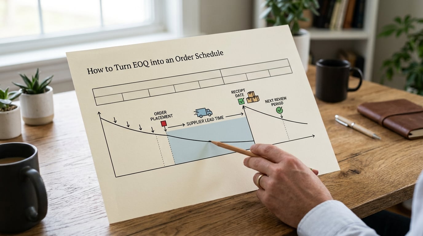
For the packaging buyer above, lead time is three weeks. Demand during lead time is 48,000 ÷ 52 × 3 = 2,769 units. Add 500 units of safety stock for late print runs and the reorder point lands at 3,269 units on hand.

So the policy reads: when inventory on hand for a line falls to 3,269 boxes, raise a PO for 9,750. Receipt is about three weeks later, when on-hand has dipped to roughly 500 units. Simple, repeatable, and it does not need a person to make a judgement call every Friday.

Two scheduling styles exist. Continuous review means you watch on-hand levels and order the moment you cross the trigger. Periodic review means you count on a fixed day — weekly or monthly — and order for the period plus lead time. Under periodic review, the reorder point carries the whole review period as well as lead time, so it is always higher.

Recalculate the reorder point when lead time changes, not just when demand does. A supplier moving from three weeks to eight added 1,155 units of lead-time demand in this example, which is a bigger shock than most buyers expect.

When a Buyer Should Not Use the Standard EOQ

The basic EOQ model assumes constant demand, constant lead time, instant receipt and no shortages. Real purchasing breaks most of those assumptions, and a few situations break them badly enough that the number is misleading.

Nonconstant demand. If monthly sales swing 3x between January and December, an annual average hides the peak. Most buyers run EOQ on average demand and then add a seasonal overlay on top.

Perishables and short shelf lives. Holding cost is not a percentage of value when the goods expire. Spoilage, markdown and disposal replace the storage line, and the holding rate you use becomes the dominant term in the formula.

Seasonal and fashion goods. Last season’s colourway has no value at all, so obsolescence risk is closer to 100 percent of unit cost than the 4 percent line item most buyers assume.

Long and variable lead times. A twelve-week ocean lead that stretches to twenty destroys the reorder point even when the quantity is right. Lead time variability belongs in safety stock, not in the EOQ figure.

Custom-manufactured components. When the supplier builds to your order, the holding cost of raw material before installation is not comparable to a stocked finished good. Setup cost per lot is a better lever than quantity.

Thin cash and multi-SKU catalogues. A thousand-SKU catalogue cannot have nine thousand EOQ numbers. Buyers apply ABC analysis first and calculate EOQ only for A and B items, managing C items on a simple min-max rule.

How to Adjust EOQ for Real Purchasing Conditions

The calculated number is a starting point. Real purchasing adds constraints on top of it, and the trick is adjusting inputs rather than rewriting the answer.

Supplier minimum order quantity. If EOQ comes out at 4,000 units and the MOQ is 10,000, you have three choices: buy the MOQ and hold more, find a second supplier, or negotiate. A useful test is total cost at the MOQ versus total cost at EOQ. If the difference is smaller than the cash strain of holding 10,000 units, buy the MOQ and manage the risk. EOQ below the MOQ is also real negotiating leverage, because it is a number, not a preference.

Case packs. Round up to the next full case, then divide the real holding cost by the whole order. Rounding up by a few units is the one adjustment that does not need recalculating.

Quantity discounts. Work out total annual cost at each break price: purchase cost of D units plus ordering cost of D ÷ Q orders plus holding cost of Q ÷ 2 units. Pick the lowest total, not the biggest discount. An all-units discount makes the larger quantity genuinely cheaper, while an incremental discount often does not survive the freight and warehousing it triggers.

Freight and cost changes. A jump in fixed per-shipment costs raises S, which pushes quantity up. A rise in variable freight per box is part of unit cost and enters through H. Putting variable freight into S double counts it and inflates your order size.

Holding rate sanity checks. Between 20 and 30 percent of unit value per year is a common band for a small business with real storage and insurance. A 5 percent rate usually means capital cost was left out, which quietly pushes the recommended quantity down.

How to calculate EOQ in a spreadsheet

There is an EOQ formula in Excel, and it is a single function once the inputs sit in their own cells. Put annual demand in B2, ordering cost in B3, unit cost in B4 and the holding rate in B5. B6 is H: =B4*B5. B7 is the answer: =SQRT(2*B2*B3/B6). B8 rounds it: =ROUND(B7,0). B9 gives orders per year with =B2/B8, and B10 gives cash sitting in cycle inventory with =B8/2*B4.

Copy that block down one row per SKU and add columns for MOQ, case pack and lead time. Then the adjustment rules above become spreadsheet logic rather than arithmetic you redo by hand each quarter.

EOQ Versus Minimum Order Quantity and Reorder Point

EOQ, MOQ and the reorder point are three different numbers that buyers constantly blur together. Here is the clean split.

EOQ compared with MOQ, reorder point and safety stock

	EOQ	MOQ	Reorder point	Safety stock
Question it answers	How much to order	How little you can order	When to order	How much buffer to hold
Who sets it	You, using your own cost data	The supplier	You, from lead time and demand	You, from lead time variability and service level
Units	Units per order	Units per order	Units on hand	Units on hand
Calculation	√(2DS ÷ H)	Supplier policy, often per colour or per size	Demand during lead time plus safety stock	Service level times demand variability during lead time
Common mistake	Treating it as an order date	Assuming your EOQ is negotiable on its own	Setting it below safety stock	Padding it with uncertainty that belongs in the forecast

EOQ and reorder point are a pair: the reorder point is the trigger, EOQ is the payload. MOQ is an external constraint, and a buyer who has never computed EOQ cannot negotiate against one with any credibility.

Key Assumptions and Common Calculation Errors

A valid EOQ result needs constant demand, constant lead time, instant receipt of the full order, no shortages allowed, and a stable unit cost. When those hold, the formula is genuinely useful. When they do not, the output is a starting estimate at best.

The errors I would check first, in order of how often they appear:

1. Mixed time units. Monthly demand against a yearly holding cost. Multiply by twelve and multiply the holding rate by twelve, on both sides.

2. Unit cost used as holding cost. H is a per-year carrying amount, not a purchase amount. Using 0.38 where 0.0836 belongs makes the recommended quantity roughly 2.1x too small.

3. Ordering cost set to zero. It looks like a rounding error and it is not. A zero S sends the result to infinity, which is why “just order more” is so common in spreadsheets that were never finished.

4. Stale demand. Using a figure from two years ago because it is the one in the last deck. Recompute D from the last twelve months of actual issues.

5. Ignoring MOQ and case packs. The formula result is not the quantity you can actually buy.

6. Treating EOQ as a recommendation to buy. It is a sizing input. Whether to buy at all depends on cash, capacity and whether the item is even worth stocking.

One more judgment call: not every SKU deserves the work. Under ABC analysis, roughly the top 20 percent of SKUs often carry most of the annual value, and those are where an EOQ policy pays for itself. The long tail is better served by a simple reorder rule and periodic review.

A Buyer-Friendly EOQ Workflow

Pulling this together as a process, so it survives contact with a busy week:

1. Pick the items. Start with your A and B SKUs, not the whole catalogue. Ten lines done properly beat four hundred done approximately.

2. Measure D. Twelve months of actual units issued, with any one-off spikes flagged and explained.

3. Build S from your own time. Time the last five POs end to end, from writing the order to putting the goods away, and price that time. Add fixed freight and documentation per inbound shipment.

4>Build H from real percentages. Capital at your borrowing rate, storage and insurance from your actual invoices, shrinkage and obsolescence from last year’s write-offs.

5. Calculate and test neighbours. Run the number, then run half and double. If the total cost barely moves, your inputs are not sensitive and you can stop arguing about decimals.

6. Apply constraints. Round to case pack, respect MOQ, check discount tiers, and set the reorder point from lead time plus safety stock.

7. Write it down and review it. Put the policy in a one-page document with the assumptions listed, then recalculate quarterly and whenever lead time or demand shifts materially. Compare the actual orders you placed against the policy and note the gap.

That last step is the one teams skip, and it is the one that turns a spreadsheet into a policy that improves.

Frequently Asked Questions

Conclusion: Start with a Testable EOQ Policy

Economic order quantity explained for buyers boils down to four numbers you can defend: annual demand, ordering cost per order, holding cost per unit per year, and the supplier constraints sitting on top of them. Validate all four before letting the formula set an order size.

Start with your ten highest-value SKUs, time one real purchase order end to end, and pull last year’s write-offs. That single afternoon usually surfaces more savings than any discount negotiation, because the numbers that come out of it are the ones you can actually use when a supplier pushes back on quantity.