

Safety stock is the inventory you hold beyond what you expect to use before the next delivery lands, so demand spikes and supplier delays never turn into a stockout. There are two ways to calculate safety stock levels, and which one you pick depends on the data you have. Both formulas below are worth knowing.
Formula: Safety stock = (maximum daily sales x maximum lead time) – (average daily sales x average lead time)
Formula: Safety stock = Z x sigma (standard deviation of demand) x square root of the lead time
Use the first when you only have simple sales and delivery records. Use the second when you can measure variability properly and hold a specific service target. Once the number exists, the reorder point is easy: average demand during lead time, plus the safety stock figure.
The whole job takes about an hour per SKU if your data is clean. The awkward part is rarely the arithmetic, it is deciding what counts as your average and your maximum, and being honest about the service level you are paying for.
Table of Contents
- What You Need Before You Start
- How to Calculate Safety Stock Levels Step by Step
- Common Mistakes When Calculating Safety Stock
- Frequently Asked Questions
- Is safety stock the same as the reorder point?
- What service level should a small business target?
- How do I calculate safety stock for intermittent demand?
- How do I set safety stock for perishable or seasonal products?
- How do I handle multiple suppliers with different lead times?
- What is the best way to run this calculation in a spreadsheet?
- Conclusion
What You Need Before You Start
To calculate safety stock levels you need a demand history, a lead-time history, and a target service level. How to calculate safety stock levels well comes down to stating those inputs precisely, because most disagreements about the result are really disagreements about the window and the units.
- Average demand. Units used per day over a stated period, for example the last 90 days. The period must be written down, or two planners will produce two different numbers from the same system.
- Demand variability. The standard deviation of daily demand over that same period. This is the number most guides skip and the one that matters most.
- Average lead time. Days from purchase order to receipt, averaged across every order you placed in the window.
- Lead-time variability. The standard deviation of those same lead-time days. If your supplier is a wildcard, this can be as important as demand variability.
- Target service level. The share of replenishment cycles you want to finish without a stockout, expressed as a percentage and converted to a Z-value.
- Review period. How often stock is checked. In a continuous review it is zero; in a weekly count it adds a week of protection.
- Inventory position. On hand, minus backorders, plus anything already on order. This is the figure the reorder point is tested against.
- Reliable history. At least 90 days for a stable item, a full year for anything seasonal, and enough purchase orders to average lead time.
All of this normally lives in your POS, ERP or WMS already. If it does not, start by exporting daily sales by SKU and PO date against receipt date, because those two columns produce every input you need.
How to Calculate Safety Stock Levels Step by Step
1. Define the Inventory Objective
Before any formula, write down the item, the location, the demand pattern, how it gets replenished, and what a stockout actually costs you. A packaging component on an assembly line with a two-hour downtime cost per hour is a different problem from a retail accessory that can be reordered tomorrow.
Keep four inventory terms apart, because mixing them is where most spreadsheets go wrong:
- Cycle stock is the quantity you deliberately order to cover demand between replenishment points, usually half an order quantity under an economic order quantity policy.
- Safety stock is the buffer above cycle stock, held only to absorb uncertainty. It is not ordered for a reason you can name.
- Reorder point is the inventory position that triggers a new order. It is a trigger, not a quantity of buffer.
- Average inventory is roughly cycle stock plus half your safety stock, and it is what carrying cost gets applied to.
Write the objective as a sentence. “Hold 20 days of cover on this component because an unplanned stoppage costs more than the extra carrying charge” is useful. “Keep some extra” is not.
2. Calculate Average Demand
Average demand is total units used in the period divided by the number of days in the period, using one consistent unit throughout. Mix cases and eaches, or shipments and orders, and the mean becomes fiction.
State the window in the spreadsheet itself. For a stable item, the last 90 days of daily usage is a reasonable default because it captures recent behaviour without seasonal bias. For seasonal products, use a full year and pull the demand from the matching season rather than averaging across all of it.
Also record peak demand, not just the average. The basic formula needs the maximum, and the maximum tells you something useful even when you use the statistical method, because a gap between your busiest day and your typical day is a forecast problem worth fixing upstream.
3. Measure Demand and Lead-Time Variability
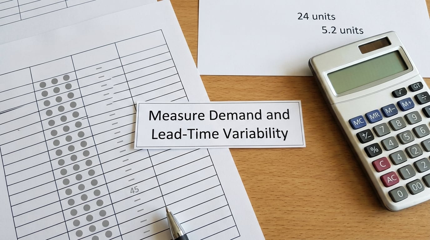
Standard deviation is the spread of your data around its mean, and it is the single input that turns a guess into a calculation. If daily usage over 90 days runs between 4 and 36 units, the standard deviation tells you how much of the demand swing is normal and how much is exceptional.
To calculate the inputs in a spreadsheet, lay your data out in columns and use these functions:
- Average daily demand:
=AVERAGE(B2:B91)on 90 rows of daily sales - Maximum daily demand:
=MAX(B2:B91) - Standard deviation of demand:
=STDEV.S(B2:B91) - Lead-time days per order:
=C2-B2, receipt date minus PO date - Average lead time:
=AVERAGE(E2:E26) - Maximum lead time:
=MAX(E2:E26) - Standard deviation of lead time:
=STDEV.S(E2:E26)
The classic combined variability measure used in the safety stock formula is the square root of the sum of the two variances, demand variance plus lead-time variance multiplied by average demand, written as the square root of (L x sigma squared + D squared x sigma-LT squared). With reliable lead times, most planners use the simpler square root of L on demand sigma alone, and the difference is usually small.
One caveat worth knowing: demand and lead time are often correlated, because large orders tend to take longer. Every formula here assumes they move independently. If your supplier slows down exactly when you ramp up, add a judgement buffer on top rather than pretending the maths handles it.
4. Convert the Service-Level Goal Into a Z-Value
Your service level is the probability of not stocking out during a replenishment cycle, and it converts into the multiplier Z in the formula. A cycle service level of 95% means roughly 19 cycles in 20 finish without running out, which is not the same promise as a 95% fill rate across all order lines.
Use the standard normal table or the equivalent Excel function =NORM.S.INV(0.95). These are the values you will use most:
| Target service level | Z-value | What it means in practice |
|---|---|---|
| 90% | 1.28 | About 1 stockout in 10 cycles; occasional backorders get handled by expediting |
| 95% | 1.65 | The common default; 1 stockout in 20 cycles |
| 97.5% | 1.96 | Two sigma, the point ASCM associates with covering about 98% of cycles |
| 98% | 2.05 | Rarely quoted, but a normal choice for contract penalty clauses |
| 99% | 2.33 | Three sigma; for items where a stockout is genuinely expensive |
Service level is a cost decision, not a preference. In the worked example below, moving from 95% to 99% adds roughly 0.68 x 12 x square root of 5, which is about 19 extra units sitting on the shelf. That is a fair trade for a high-margin item with no second source and a poor trade for a cheap part with four qualified suppliers.
5. Calculate Safety Stock Levels and Reorder Point
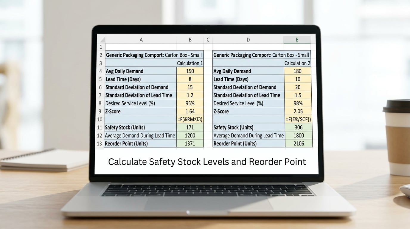
Here is the full arithmetic for a packaging component at a mid-sized manufacturer. Average daily demand is 20 units, the standard deviation of daily demand is 12 units, and average lead time is 5 days with a target service level of 95%, so Z is 1.65.
Safety stock = Z x sigma x square root of L = 1.65 x 12 x 2.236 = 44.3, rounded up to 45 units
Rounding up is the correct move. A buffer of 44 protects nothing that 45 does not, and the whole reason for holding it is the case where the arithmetic lands exactly on the boundary.
Reorder point = (average daily demand x average lead time) + safety stock = (20 x 5) + 45 = 145 units
So you place a new order the moment inventory position drops to 145 units. If cycle stock is set by an economic order quantity of 800 units, average inventory is roughly 400 plus 45, and the safety portion is a small slice of what you already hold.
For contrast, the basic average-max formula on a less predictable supplier gives a much larger answer. With average daily demand of 20, maximum daily demand of 45, average lead time of 5 days and a maximum lead time of 9 days, safety stock comes to (45 x 9) minus (20 x 5), or 305 units. That is not a mistake, it is the method behaving exactly as designed: a single worst-case day sets the whole buffer. Use it when you have no reliable variability data, and expect it to over-protect.
The 50% rule is the quick shortcut between the two. Take half the difference between maximum and average lead time, multiplied by average daily demand: half of (9 minus 5) times 20 equals 40 units. It is a reasonable middle when you have demand figures but no time to compute a standard deviation.
6. Add Review-Period and Lead-Time Considerations
If you count inventory weekly rather than continuously, an order placed after the count still waits a full week. Your protection period becomes lead time plus review period, so use 12 days instead of 5 in the square root, and the buffer rises on its own. This is the most commonly missed adjustment in periodic-review systems.
When demand is intermittent, with many days at zero and occasional large orders, a normal distribution is the wrong shape. Poisson, binomial or gamma methods handle that case better, and a simpler fallback works too: set the buffer in days of cover and multiply by average demand, then review it against actual stockouts each period. Practitioners on supply chain forums run a simplified safety-days variant quarterly for exactly this reason, and it beats a buffer that is never revisited.
7. Validate and Update the Result
Compare the calculated buffer against what actually happened: stockout frequency, backorder count, fill rate, and supplier on-time performance. If a 95% target produced five stockouts in a quarter, either the demand data is wrong, the service level is unrealistic, or the lead-time assumption is optimistic. Fix the cause, do not simply raise Z.
Quantify the other side too. Carrying cost on 45 units of a slow-moving component is trivial; the same 45 units of fast-moving finished goods is real money tied up. Then set a cadence: quarterly for stable items, monthly for volatile ones, and immediately after any supplier change, new product launch, or shift to a different distribution channel.
For seasonal items, do not inflate sigma blindly. Pull the variance from the same months last year instead, and keep two buffers, one for peak and one for off-peak, rather than one number stretched to cover both.
Common Mistakes When Calculating Safety Stock
- Using average demand with no variability. A buffer built on the mean assumes demand never surprises you, which is the one thing that makes buffers necessary. Fix: at minimum, use the 50% rule or the average-max method.
- Mixing demand and sales units. Cases and eaches, or shipped units and ordered units, quietly halve your buffer. Fix: convert everything to a single stock-keeping unit and write the unit next to the number.
- Applying one target to every SKU. A single service level applied to a thousand items is either ruinously expensive or useless. Fix: segment with ABC for value and XYZ for predictability, then set targets per segment.
- Ignoring supplier lead-time risk. Standard deviation of demand alone assumes deliveries land when promised. Fix: include lead-time variance in the combined measure, and add a manual buffer for a supplier you do not trust.
- Double-counting safety stock. Adding a buffer to an order quantity that already includes it, or counting the same units at both branch and distribution center. Fix: define safety stock once per item per location and treat inventory position as the single trigger.
- Never updating the assumptions. A buffer calculated eighteen months ago still claims to represent a supplier and a demand pattern that no longer exist. Fix: tie the recalculation to a date and to events, not to memory.
- Using the buffer for routine reorders. Pulling safety stock down to fix a missed reorder trains buyers to order earlier and inflates the real requirement. Fix: reorder on the reorder point, and treat stockouts as a data problem to investigate.
Frequently Asked Questions
Is safety stock the same as the reorder point?
No, they answer different questions. Safety stock is a quantity of extra inventory you hold. The reorder point is a trigger level: when inventory position falls to that number, you place a new order. The reorder point equals average demand during lead time plus your safety stock, so the buffer is one of the two parts that make it up.
What service level should a small business target?
Most small operators start at 95%, which allows roughly one stockout in twenty cycles, then adjust. Raise the target for high-margin items with a single supplier and no substitute. Lower it for cheap, replaceable or slow-moving goods where backorders cost little. Revisit the number once you have a quarter of actual stockout data to compare against.
How do I calculate safety stock for intermittent demand?
Intermittent demand, with many zero days and occasional large orders, breaks the normal distribution assumption behind the standard formula. Either use a distribution designed for that pattern, such as Poisson, or set the buffer as a set number of days of cover multiplied by average demand. Whichever you choose, review it against actual stockouts each period.
How do I set safety stock for perishable or seasonal products?
For seasonal items, calculate variability from the matching months last year rather than across a full year, and keep separate peak and off-peak buffers. For perishables, the service level matters less than shelf life: holding enough to hit 99% is pointless if the units expire. Cap the buffer at a fraction of remaining shelf life.
How do I handle multiple suppliers with different lead times?
Calculate a separate buffer for each source, using that supplier’s own lead-time history rather than a blended average, and set the reorder point against the source you will actually use next. If you switch sources frequently, add a switching buffer on top. Weights on the sources do not change the arithmetic; only the reliability assumption does.
What is the best way to run this calculation in a spreadsheet?
Keep one row per SKU per period with daily demand and a separate lead-time column, then use AVERAGE, MAX and STDEV.S on those columns and NORM.S.INV to look up the Z-value. That structure means each new period is an appended row, not a rebuild, and the buffer updates with a fill-down formula.
Conclusion
Start with the method that matches your data, not the one that gives the answer you want. Pick a service level, calculate the standard deviation of demand and lead time in your spreadsheet, multiply Z by sigma by the square root of lead time, then add average demand during lead time to reach the reorder point. Check the result against last quarter’s stockouts and holding costs, and write the recalculation date on the sheet. Once you know how to calculate safety stock levels this way for one SKU, the same five steps scale to the rest of your catalogue through segmenting rather than a single blanket buffer.
Reviewed for accuracy in October 2026.